What Does Continual Learning Actually Forget? Probing Memorization vs Generalization in Sequential Training

01 — ProblemWhat Does CL Actually Erase?

Continual learning research has always measured one thing: task performance. Can the model still solve Task A after training on Task B? This is the standard metric — backward transfer, forgetting rate, plasticity-stability tradeoff. It is a reasonable proxy, but it is incomplete.

Task performance captures generalized knowledge — the model's ability to solve a class of problems. It says nothing about a second type of knowledge living in the same weights: memorized knowledge — specific data points encoded verbatim during training. A model can forget how to perform a task while still having specific examples from that task memorized. Or it can perform well through generalization with no memorization at all. These are distinct phenomena. CL research currently has no tool to distinguish them.

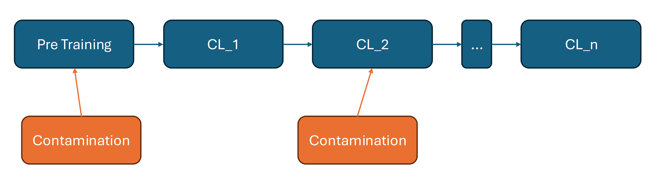
This gap has a practical edge. Contamination detection — identifying whether a model was trained on benchmark test data — depends entirely on memorization signals surviving in the model's weights. If a model is contaminated at one training stage and then continues learning, do those signals persist? Do they decay? Does it depend on how the model is trained? Nobody has studied this.

02 — MotivationWhy This Gap Matters

For CL researchers, this opens a new diagnostic dimension. EWC, replay buffers, and LoRA adapters are compared on task performance alone. But they may treat memorized and generalized knowledge completely differently. EWC protects weights important for task performance — does it also protect memorization? Replay literally replays training data, which should strongly preserve memorization signals. LoRA freezes base model weights entirely — contamination stored there cannot be touched by new task adapters. Each method reveals something different about where knowledge lives in weight space, but only if you have a probe sensitive enough to distinguish memorization from generalization.

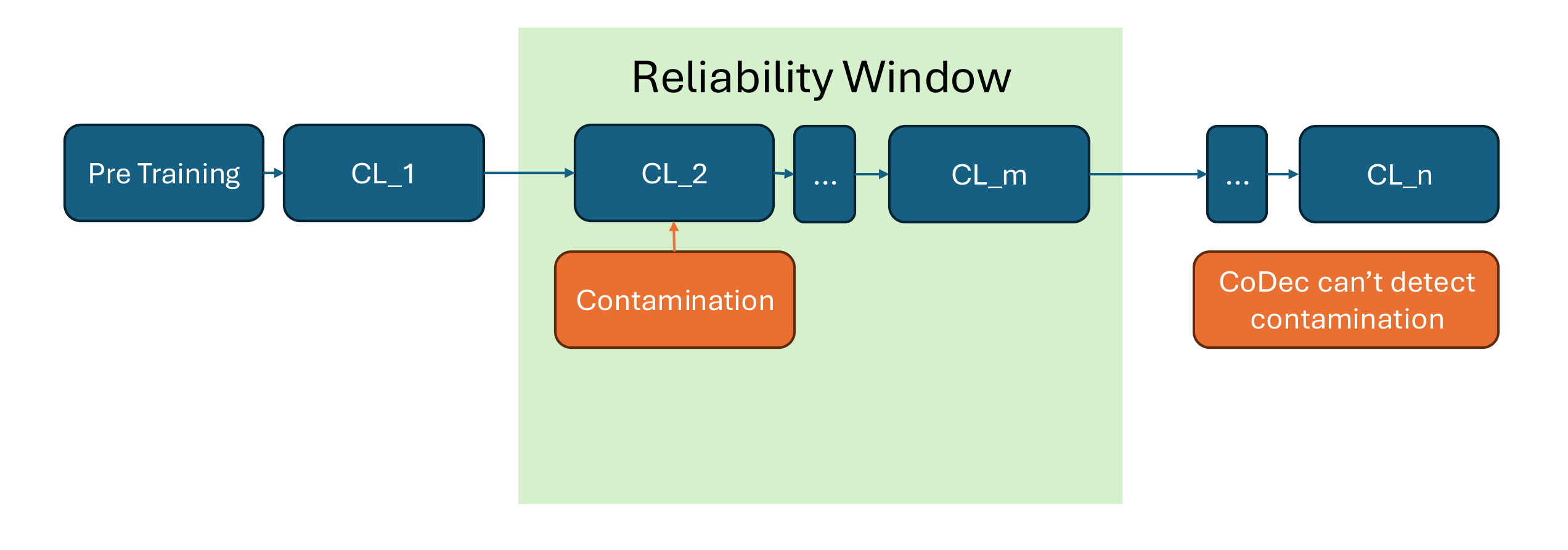
For auditing deployed models: a model trained at stage A, then updated at B, C, and D — can you still detect that stage A introduced contaminated data? For how long does the signal survive? Is there a point of no return? These questions determine whether retrospective auditing is even possible, which matters for anyone deploying models that learn continuously.

03 — ApproachCoDec as Probe, LMC as Explanation

This research uses two tools in combination: CoDec as the measurement instrument and Linear Mode Connectivity (LMC) barriers as the geometric explanation.

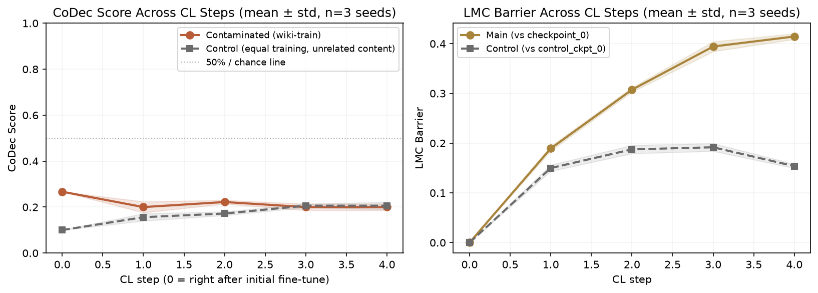
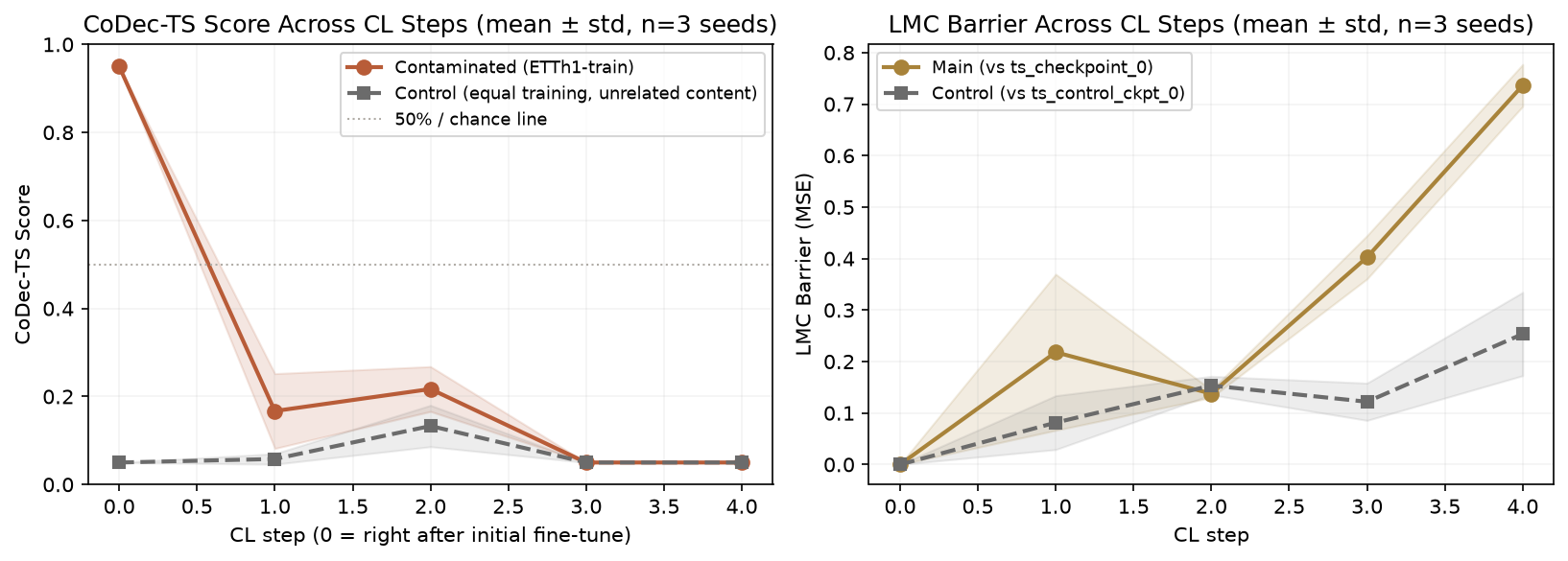
CoDec (Zawalski et al., ICLR 2026) detects memorization by exploiting a behavioral asymmetry. For data the model has never seen, in-context examples help — they provide useful signal. For data the model has memorized, in-context examples disrupt — the model already knows the answer and gets confused by seeing it reframed. The CoDec score is the fraction of test samples where adding context decreases the model's log-probability. High score (>80%) indicates contamination; low score (<50%) indicates clean data.

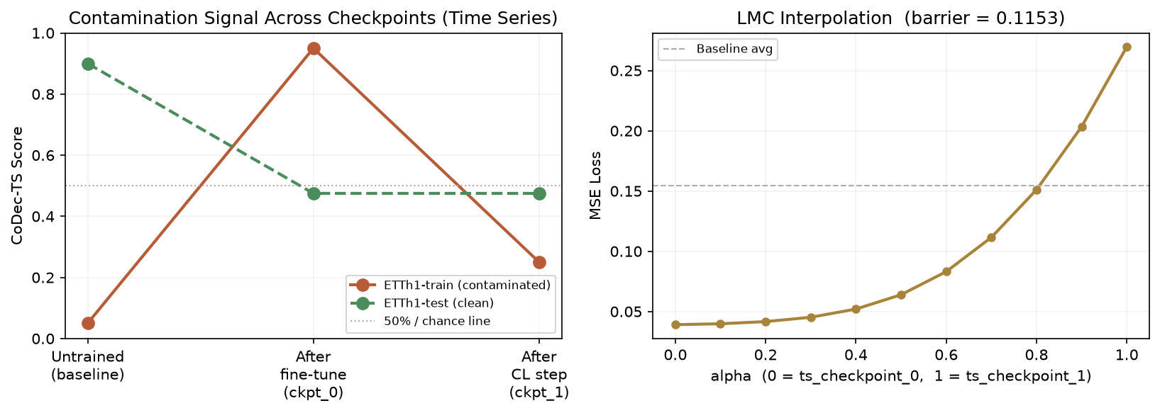
LMC barriers measure whether two model checkpoints occupy the same loss basin. A low barrier means a low-loss linear path exists between them in weight space — they are geometrically close. A high barrier means the model has moved into a different region. The hypothesis: CoDec signals persist as long as the model stays in the same basin as the contaminated checkpoint. When CL training crosses a basin boundary, the memorization signature collapses. If this holds, LMC barriers are a leading indicator of signal decay — detectable without needing the contaminated benchmark at all.

04 — PoCBaseline Already Running

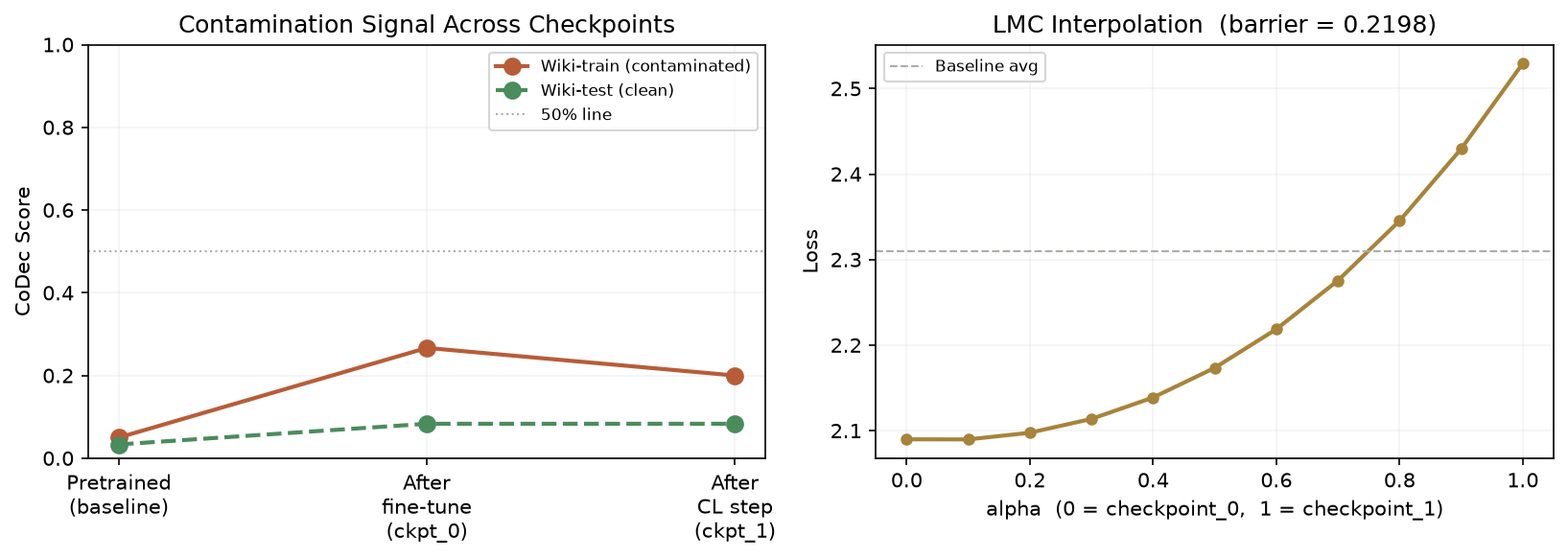
To establish the baseline, I fine-tuned GPT-2 (117M) on a held-in text corpus and measured CoDec scores on that corpus versus a clean held-out set. This confirms the signal is detectable at this scale and that the re-implementation of CoDec matches the paper's behavior. The research question is what happens to the contaminated score as the model continues training on sequential unrelated tasks.

05 — Research QuestionsFive Questions That Form the Thesis

• 01 Do CL methods erase memorized and generalized knowledge at the same rate, or differently? Answered by plotting task performance and CoDec score on the same axis across sequential training stages.
• 02 Is LMC basin structure the geometric explanation for when memorized knowledge is lost? If barrier rise precedes CoDec decay, the model's departure from its original basin predicts signal loss — a mechanistic account, not just an observation.
• 03 Is signal decay gradual, sudden, or task-dependent? A phase transition at a specific CL step would suggest basin crossings are discrete events. Gradual decay would suggest memorization shares weights with task knowledge modified linearly by CL.
• 04 Which CL methods distinguish between memorization and generalization — and which treat them identically? EWC, replay, and LoRA adapters each constrain weight updates differently. Their behavior on CoDec vs task performance reveals what each method structurally preserves.
• 05 Can you trace which training stage introduced memorization? Given checkpoints after each stage, does differential CoDec scoring correctly attribute contamination to the right stage — and does adding LMC barrier data improve that attribution?

06 — Experimental PlanThree Experiments, Increasing Depth

07 — RisksWhat Could Go Wrong and Why It Is Still Fine

# CoDec score: fraction of samples where context DECREASES confidence
# High score = model disrupted by context = memorized data
# Low score  = model helped by context   = unseen data

import torch
from transformers import GPT2LMHeadModel, GPT2Tokenizer

def logprob(model, tokenizer, text, context=None, device="cpu"):
    prompt  = (context + "\n\n" + text) if context else text
    ctx_len = len(tokenizer(context + "\n\n").input_ids) if context else 0
    ids     = tokenizer(prompt, return_tensors="pt").input_ids.to(device)
    with torch.no_grad():
        loss = model(ids, labels=ids).loss
    return -loss.item()

def codec_score(model, tokenizer, samples, k=3, device="cpu"):
    disrupted = 0
    for i, x in enumerate(samples):
        context  = " ".join([s for j, s in enumerate(samples) if j != i][:k])
        lp_plain = logprob(model, tokenizer, x, device=device)
        lp_ctx   = logprob(model, tokenizer, x, context=context, device=device)
        if lp_ctx < lp_plain:
            disrupted += 1
    return disrupted / len(samples)

# Barrier > 0: loss hill exists between checkpoints = different basins
# Barrier ~ 0: low-loss path exists = same basin

def lmc_barrier(model_a, model_b, eval_fn, steps=11):
    """eval_fn: takes a state_dict, returns scalar loss"""
    loss_a   = eval_fn(model_a.state_dict())
    loss_b   = eval_fn(model_b.state_dict())
    baseline = (loss_a + loss_b) / 2
    max_loss = baseline

    for alpha in torch.linspace(0, 1, steps):
        a = alpha.item()
        interp = {
            k: (1 - a) * model_a.state_dict()[k] + a * model_b.state_dict()[k]
            for k in model_a.state_dict()
        }
        max_loss = max(max_loss, eval_fn(interp))

    return max_loss - baseline

conda create -n poc python=3.11 -y
conda activate poc
pip install torch transformers datasets matplotlib

# GPT-2 117M fits in CPU RAM
# Fine-tuning 200 examples: ~10 min on CPU
# All claims scoped to GPT-2 scale; larger models are upside if compute allows